Regularization
I am back after some time. I have been working in a startup called PerfectRec, and the work there has been ML-heavy. I am their “expert” on learn-to-rank, and learning / reading up on literature has motivated me to get back to blogging. Anyways, let’s get started!
Much of the below content is taken from my recent readings from this Wikipedia page and from [1], and it additionally includes some of my speculations / thoughts. But I’m thinking this post will be on the lighter / simpler end of what I’m planning to write for future posts. It doesn’t go deep into the theory, but I felt the ideas still might be worth sharing!
Linear Regression: Problem Statement
The least-squares linear regression can formally be stated as follows:
\[\arg\min_{\beta}\frac{1}{N}||b - \beta^Tx||_2^2\](one can assume here that \(b, \beta^T \in \mathbb{R}^d, x \in \mathbb{R}^n\)), i.e. we want to find a \(\beta\) such that the least squares error for \(\beta^Tx + \beta_0 = b\) is minimal.
There tend to be issues with standard linear regression, where the function may not be the “best fit”. Especially in higher dimensions, the model tends to find functions with overly complicated strucuture, i.e. there exist functions with more zero parameters that fit the data appropriately. We ideally want a function that 1) has a simple and 2) is interpretable, i.e. one can determine which parameters are actually relevant. Below, we will introduce regularization, which serves to resolve these issues.
A Regularization example: LASSO Regression
The idea of Lasso (least absolute shrinkage and selection operator) is to solve the above optimization problem, but with an additional constraint:
\[\sum_{i=1}^d \beta_i \leq t\]We can rewrite the optimization problem as
\[\arg\min_{\beta}\frac{1}{N}||b - \beta^Tx||_2^2 + \lambda ||\beta||_1\]The last term can be replaced with a \(2\)-norm (called ridge regression) or a \(0\)-norm (called best subset selection).
\(\lambda\) is often referred to as the regularization parameter. What is the role of \(\lambda\)? One explanation that is often used (although maybe quite non-rigorous?) is that when \(\lambda\) is large, there is more penalty for making the entries of \(\beta\) large, forcing the classifiers to be simpler.
We can also discuss the following to see what happens during the regularization (in the case of Lasso).
Consider the constraint \(\sum_{i=1}^d \beta_i \leq t\). The region for feasible \(\beta\) can be seen in the shaded region in the image below (image source from [1]):
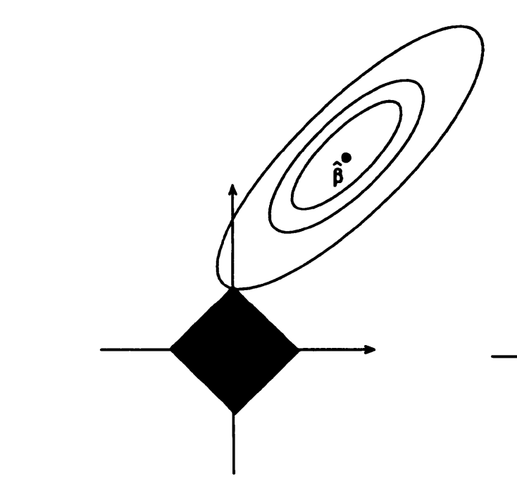
\(\hat{\beta}\) is the least-squares optimal solution, and each ring is the set of points where the loss function is equal to a certain value (note that the contours have this structure since the least-squares loss is convex). We want to minimize the loss while being within the boundary, and this will in general happen when we are at a “corner” of the boundary; i.e. the solution that is given will have a sparse structure. Having few nonzeros is advantageous in that 1) it is a simple model and will thus be less likely to overfit, and 2) the model is interpretable since we can better determine which variables (i.e. the nonzeros) have a contribution to the problem we have at hand.
Other forms of regularization
There is also \(L_2\) (ridge regression), where the constraint is an upper bound on the two-norm of \(\beta\), rather than the \(1\)-norm. One can visualize the diagram from above, except the dark region is a Euclidean ball rather than an \(L_1\) ball. The solution will not necessarily have a sparse structure anymore, but many of the coordinates will tend to be similar to each other.
There is also subset selection, which has an \(L_0\) constraint. This is generally performed by setting coordinates below a threshold to zero.
References
[1] Regression Shrinkage and Selection via the Lasso. Robert Tibshirani. Paper link
[2] Wikipedia page for Lasso Regression
[3] Wikipedia page for Ridge Regression